Introduction
In this third blog post, I want to explore how we can best use polls to predict election outcomes. I will do this through the following steps:
1) First, I am going to visualize poll accuracy over time.
2) Next, I will use various regularization techniques to create a model that will predict the 2024 election.
3) Then, I will use ensemble learning methods to combine models that incorporate both fundamental (economic) and polling data.
4) Lastly, I will discuss G. Elliott Morris and Nate Silver’s contrasting approaches when it comes to weighting fundamental and poll-based forecasts.
The code used to produce these visualizations is publicly available in my github repository and draws heavily from the section notes and sample code provided by the Gov 1347 Head Teaching Fellow, Matthew Dardet.
Analysis
First, I want to visualize polling data across years and identify whether there is a pattern for which weeks before the election (30 weeks before the election, 29 weeks before the election, 1 week before the election, etc.) are most predictive of the ultimate two-party national popular vote share of the election. I will do this by using a pre-processed, publicly available FiveThirtyEight data set of national polling averages since 1968.
I am choosing to look at 1988 because Michael Dukakis’s “death penalty” gaffe has often been cited as the death knell of Dukakis’s campaign, and I am curious if this is reflected in the polling data. I am also going to investigate 2020 and 2024 as I am very familiar with the timelines of these elections. Given that I am trying to predict the 2024 election, it seems important that I am intimately familiar with the voting trends of 2020, as these trends are the most recent and could best help me predict the outcome of 2024.
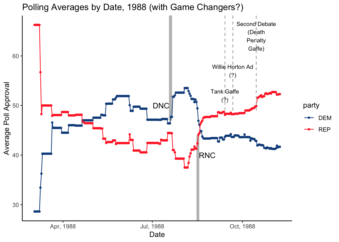
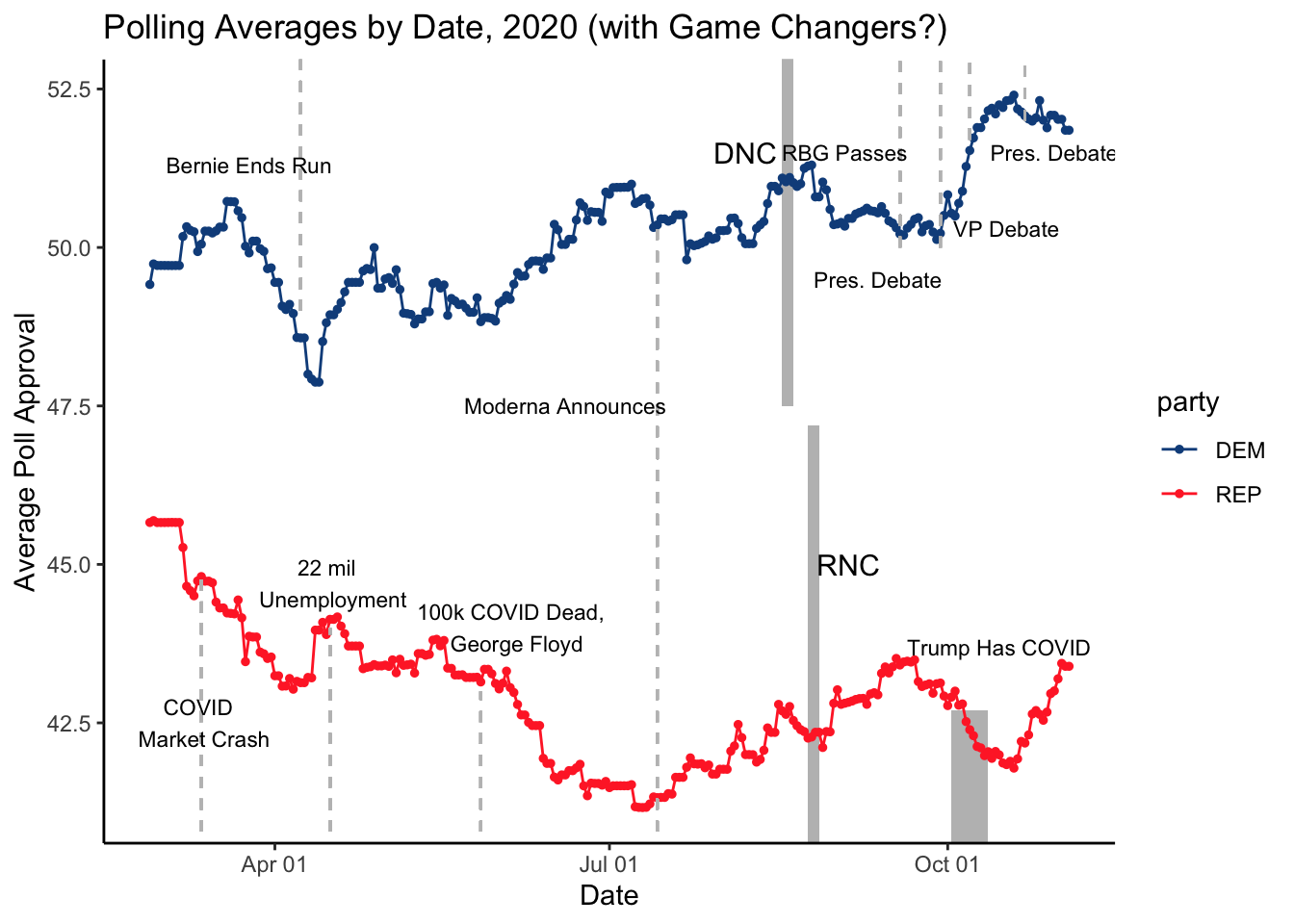
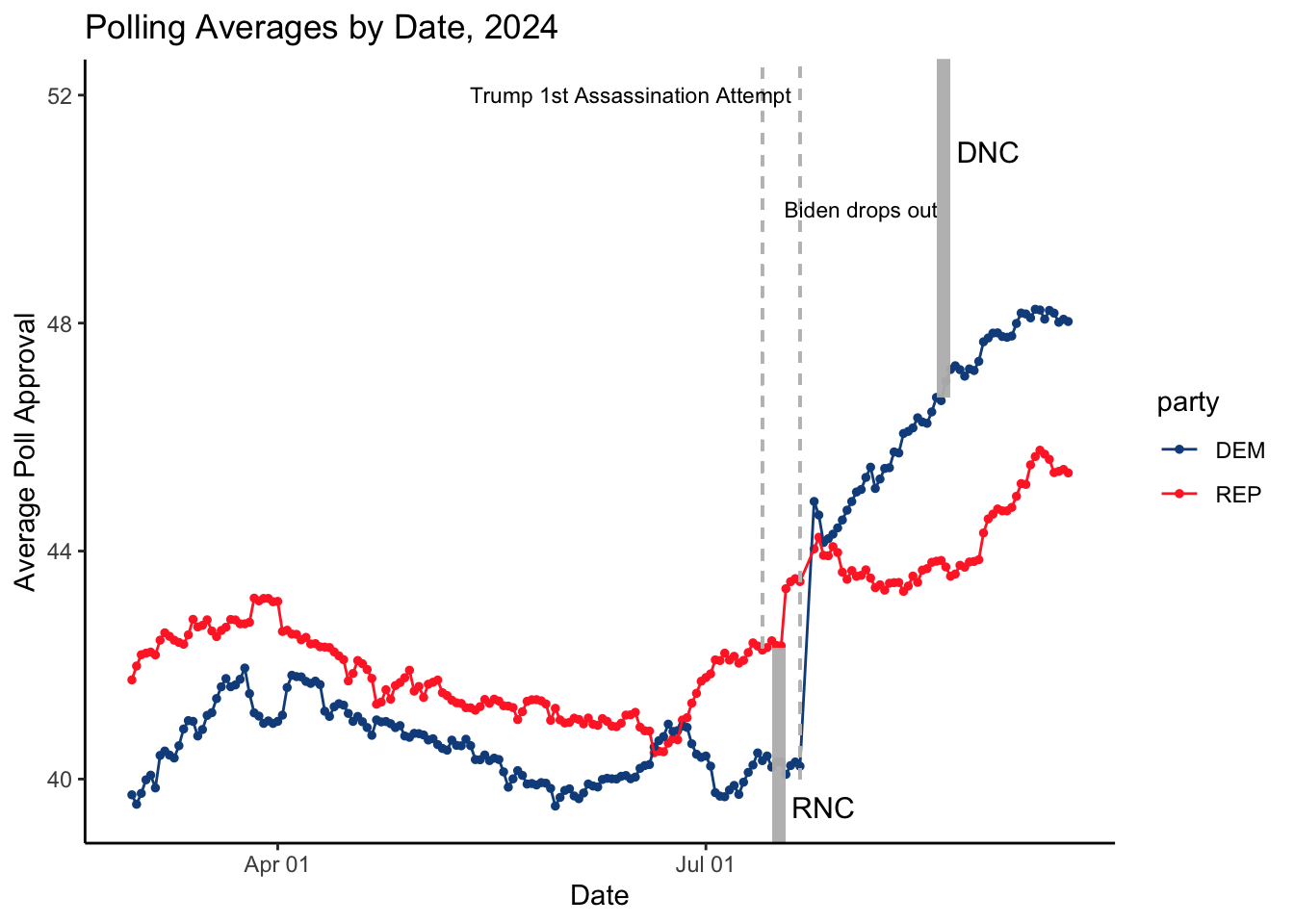
From these graphs, we can see several things.
Many of the events that pundits have characterized as determinative in elections have actually not been all that influential in candidates’ polling averages. For example, in the 1988 election, neither Michael Dukakis’s tank ad gaffe nor George H.W. Bush’s infamous Willie Horton ad had much of an effect on the polling average. The death penalty gaffe, however, did appear to offer Bush a sizeable bump in the election.
We can also see, in 2020, how the polls captured changes in voter sentiment following national emergencies and sizeable events like the COVID market crash and the George Floyd protests. Historically, each party’s national conventions tend to boost the polling average of their respective candidate, but this effect has been more muted for the Democrats in recent elections.
I also find the polling averages since 2024 to be incredibly interesting, specifically the massive boost the Democratic party experienced after Biden dropped out of the presidential election and endorsed Kamala Harris.
In order to predict the 2024 election, I am going to construct a panel of the weekly two-party national popular vote polling averages in the 30 weeks leading up to the election between 1968 and 2020. I am then going to prepare a regression that assigns a coefficient to each of these weekly polling averages. This regression will then permit me to predict the 2024 election by plugging in this cycle’s weekly polling averages so far.
In order to prevent overfitting, I will use three regularization techniques: ridge regression, LASSO regression, and elastic net regression. I will then compare these regularized approaches to the more basic OLS approach that we employed in week two.
Briefly stated, both ridge and LASSO regression employ a penalty term in the loss function that shrinks coefficients toward zero. Where OLS minimizes the sum of the squared residuals, Ridge also minimizes a penalty term that is proportional to the coefficients’ squared value. LASSO does something very similar, except its penalty term is proportional to the coefficients’ absolute value. This allows some coefficients to equal 0. Elastic Net combines both ridge and LASSO. These regularization techniques all mitigate the chance of overfitting because they preventing the calculation of large coefficients that fit statistical noise and do not consider the possibility of multicollinearity.
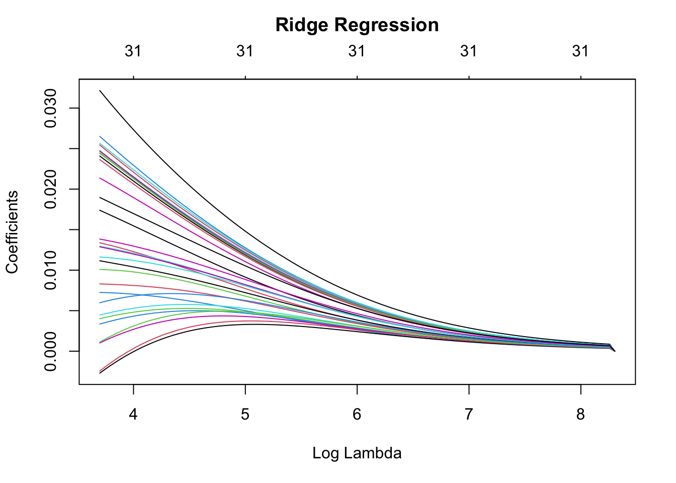
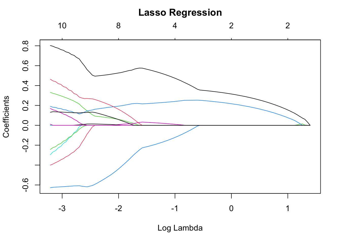
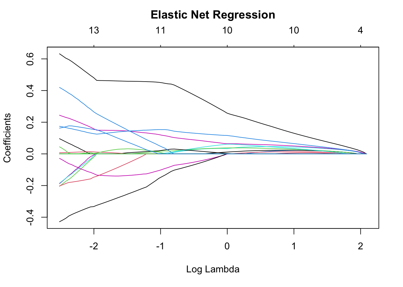
From the plots above, we see that, with a larger penalty term hyperparameter, lambda, the regression coefficients shrink toward zero faster, in the case of ridge regression, and, in the case of LASSO regression, shrink to zero faster.
By using cross-validation to minimize mean squared error, we will find an optimally predictive value for the hyperparameter, lambda, for each of the three regularization techniques. Once we do so, we observe the following coefficient plot.
Coefficient Plot
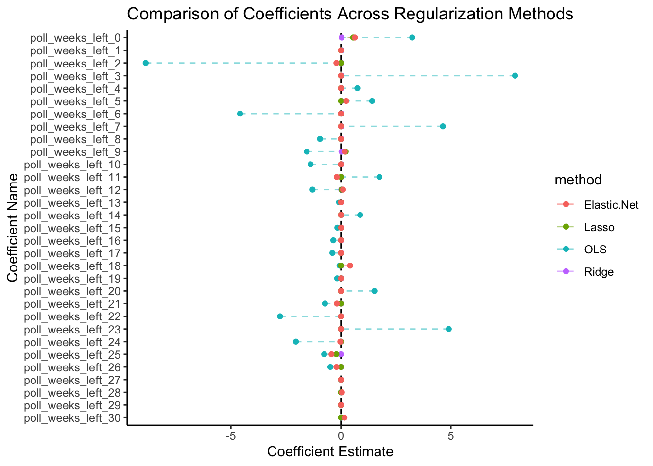
As is clear in the coefficient plot, the use of regularization techniques dramatically reduces the magnitude of the regression coefficients, perhaps reflecting the pervasiveness of the multicollinearity. Ultimately, our model suggests that the polls from the week of an election are the most important, though weeks as far back as 25 or 26 weeks before the election can still be predictive.
Using the coefficients outputted from elastic-net regression, and inputting the polling data from 2024 thus far, we find that the Democratic nominee, Kamala Harris, is projected to walk away with 51.8% of the national two-party popular vote share.
I am not wholly convinced, however, that using data from election cycles since 1968 to determine which polling weeks from 2024 will be most informative of 2024’s ultimate outcome is the best way to predict the election. Many of the coefficient values could be products of the randomness of the timing of major campaign turning points rather than reflective of any underlying patterns. My instinct tells me that polling averages become more accurate as the election looms. For this reason, I want to explore some other techniques, like ensembling that other forecasters use.
Ensembling permits us to merge the predictions of multiple models
In this section, I will prepare two models to predict 2024’s national two-party popular vote share:
An elastic net model using fundamental economic data from the Federal Reserve Bank of St. Louis.
An elastic net model that exclusively uses polling data.
I will then ensemble these models using three approaches:
Unweighted: We average the predictions from the fundamental and polling models.
Silver Weighting Approach: The weights on the polling model increase as election day nears.
Gelman & King Approach Weighting Approach: The weights on the both the economic and polling model increase as election day nears.
The polling prediction of the Democratic candidate, Kamala Harris, is listed first.
Ensemble Comparison
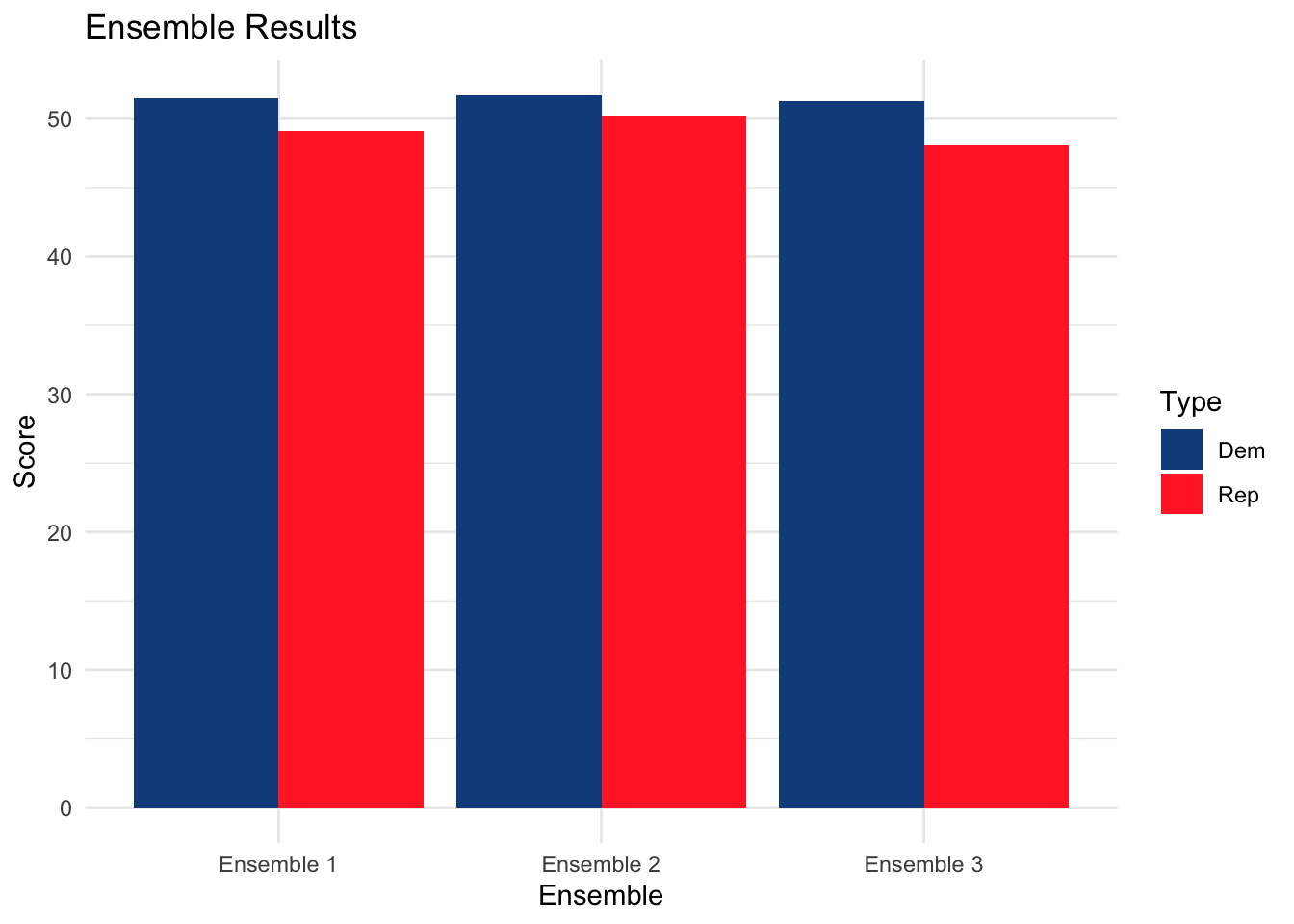
Though the ensemble prediction does not add up perfectly to 100 since we are predicting both Democratic and Republican vote share separately, we can clearly see the trend that all three ensemble models project that Harris will be the next president.
Other Methods
In recent years, two of the leading voices in election forecasting, Nate Silver and G. Elliott Morris, have publicly sparred on Twitter over their divergent approaches to weighting fundamentals and poll-based forecasts.
Silver’s Approach
Nate Silver outlines his methodology on his site, the “Silver Bulletin.”
In brief, Silver’s model prioritizes real-time polls, considering them most predictive of the actual election (and adjusting for polling bias and down-ballot effects of other races). While he does consider economic predictors and political assets like incumbency, these are secondary in importance. His model also has no current assumption about turnout for Democrats versus Republicans.
Morris’s Approach
Morris explains his philosophy on ABC’s election site, FiveThirtyEight.
Morris’s model shares many similar characteristics to Silver’s like reduced assumptions about COVID restrictions and a large emphasis on real-time polling data. Some of the most significant departures, however, are Morris’s more aggressive adjustment for conventions and his assumption about intra-region state correlation. Morris’s model also weights economic and political fundamentals more heavily, including these covariates alongside polling data rather than secondarily as Silver does.
My opinion
I personally tend to agree more with Nate Silver’s model. My impression is that Morris bakes too many of his own hunches and beliefs into the election forecast. For example, the division of the United States into correlated regions seems incredibly arbitrary and baseless to me. Likewise, Morris believes very strongly in incumbency advantage and is fairly skeptical of the polls, and, for this reason, considers polling data and political and economic fundamentals alongside one another.
I believe Nate Silver’s approach to be much more scientific. It does not allow for as much uncertainty as Morris’s and lets polls (adjusted for confidence and bias) speak for themselves as they primarily shape the model. Silver’s model, in my mind, is more objective. To me, I don’t see much need to assign much weight to electoral patterns and historic behavior when the connection between pre-election polls and actual voting outcomes are much more immediate.
Citations:
Morris, G. E. (2024, June 11). How 538’s 2024 presidential election forecast works. ABC News. https://abcnews.go.com/538/538s-2024-presidential-election-forecast-works/story?id=110867585
Silver, N. (2024, June 26). 2024 Presidential Election Model Methodology Update. Silver Bulletin. https://www.natesilver.net/p/model-methodology-2024
Data Sources:
Data are from the US presidential election popular vote results from 1948-2020, FiveThirtyEight, and the Federal Reserve Bank of St. Louis.