Introduction
In this sixth blog post, I am going to discuss the role that ads play in elections, and, then, I will discuss how a Frequentist approach to polling compares to a Bayesian approach.
I will also be updating my model from last week.
The code used to produce these visualizations is publicly available in my github repository and draws heavily from the section notes and sample code provided by the Gov 1347 Head Teaching Fellow, Matthew Dardet.
Analysis
After reading that the Harris campaign had reached over $1 billion in campaign donations,, I did a deep dive into campaign advertising throughout history.
By using data from the Wesleyan Media Project, I was able to visualize the tone of television advertisements for the presidential elections between 2000 and 2012.
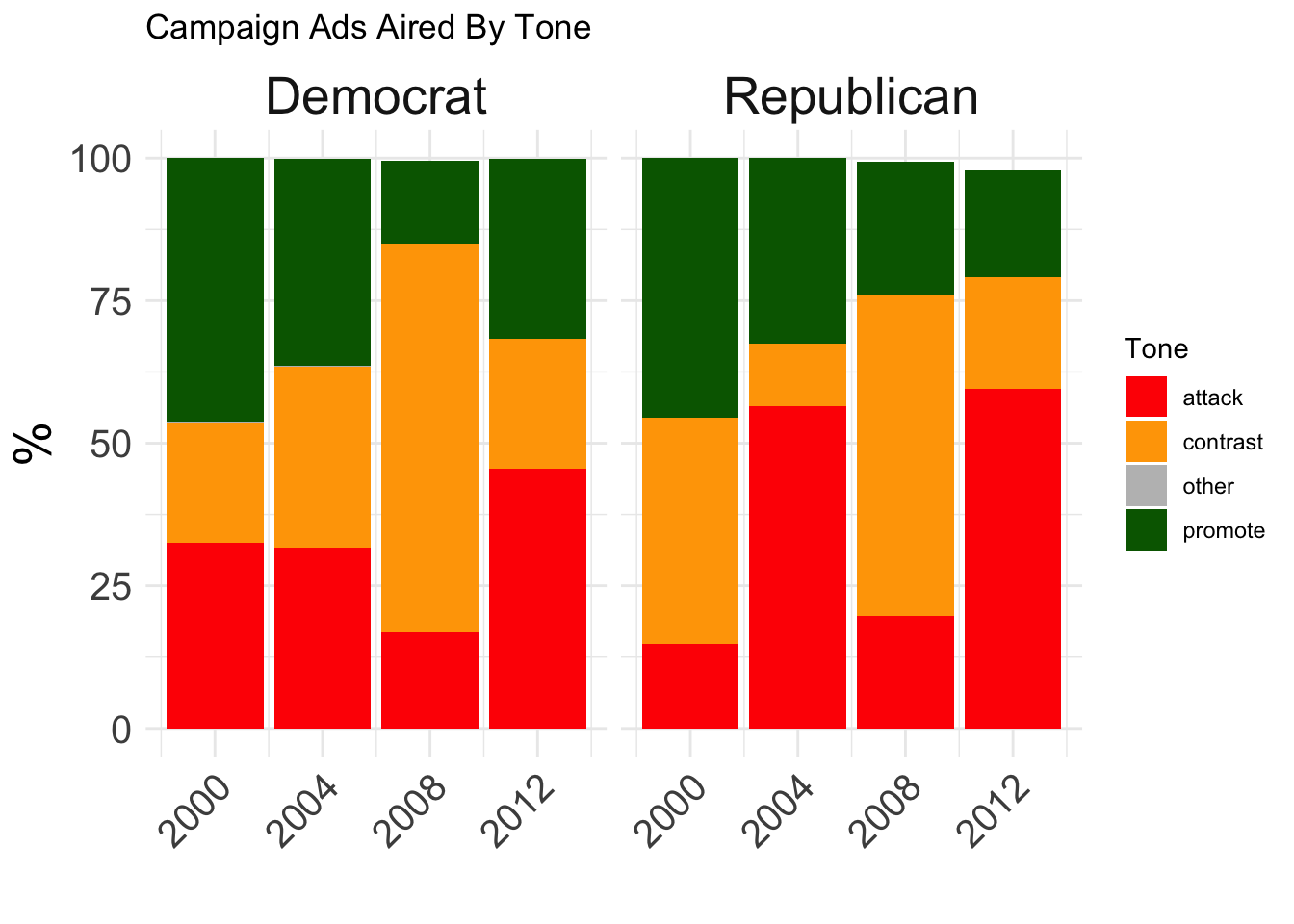
As is visible in the graph above, the election years between 2000 and 2012 saw a variety of tones within advertisements. The 2012 election cylce appeared to be pretty heated given the high incidences of “attack[ing]” tones among both candidates’ advertisements (as classified by the Wesleyan Media Project).
I will now prepare another visualization of the content of political advertisements from the same source, this time including 2016. Publicly available data only exists up until 2012, so I am using non-public data to provide the estimates for 2016.
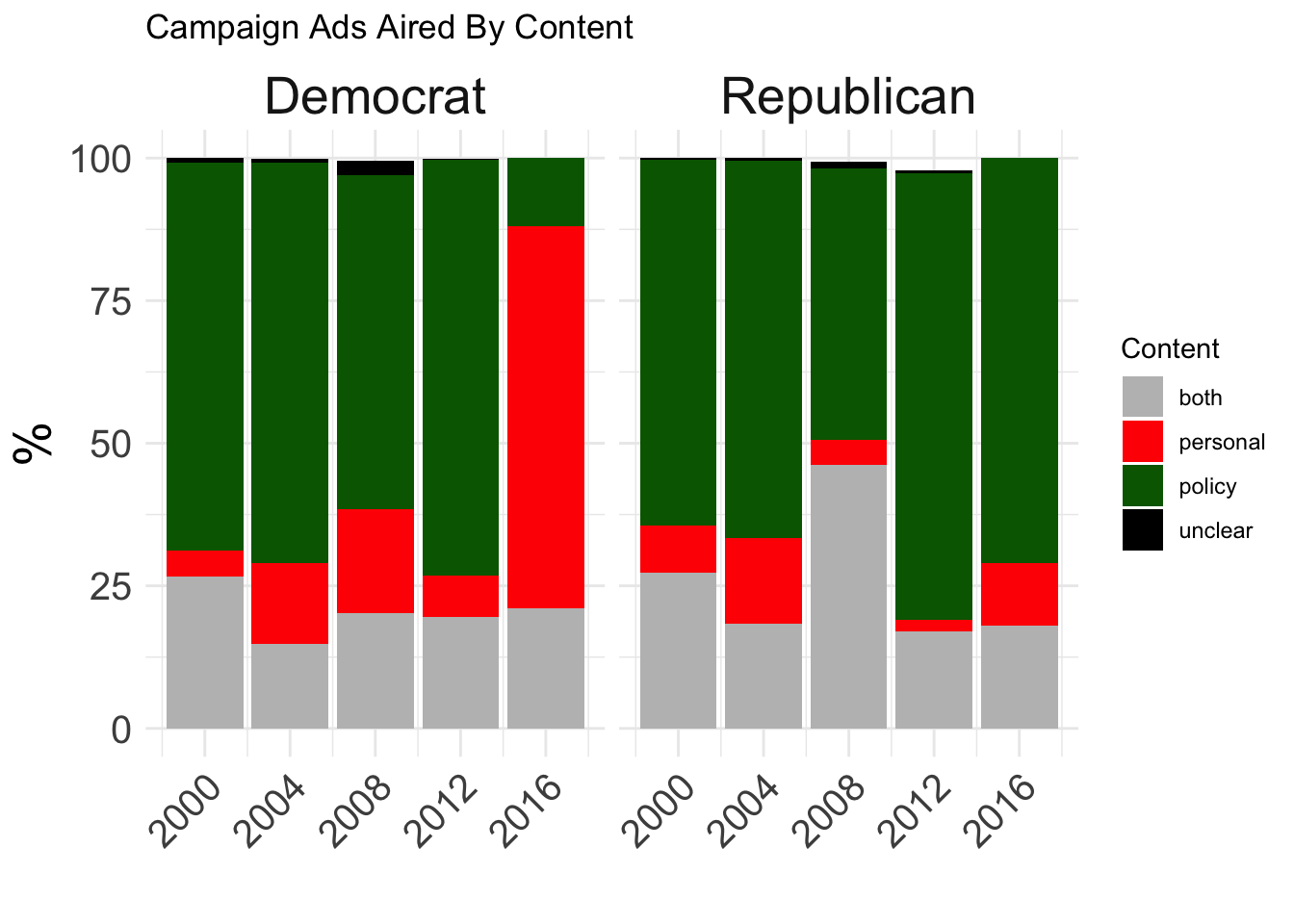
Immediately striking from this graph is the high incidence of “personal” content from the Democratic aisle in 2016. Many have noted this as the Clinton campaign’s most significant mistake: her insistence on criticizing the language, behavior, and character of Trump to voters at the potential expense of clearly articulating and evidencing her policy positions
The following graph explores the 2012 election and, for a variety of topics, the breakdown of the percentage of ads discussing those topics aired by each party.
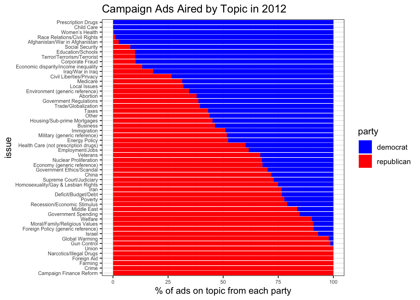
Though this election took place in 2012 in a pre-MAGA America, many of the basic dynamics between the Democratic and Republican parties still remain. For example, Republicans remain more likely to air ads on crime and Democrats more likely to air ads on child care, though it is interesting that immigration ads appear evenly split between both parties — a subject that has become much more partisan and racially charged since 2012.
Now, I am going to prepare two more graphs that evaluate campaigns’ election spending.
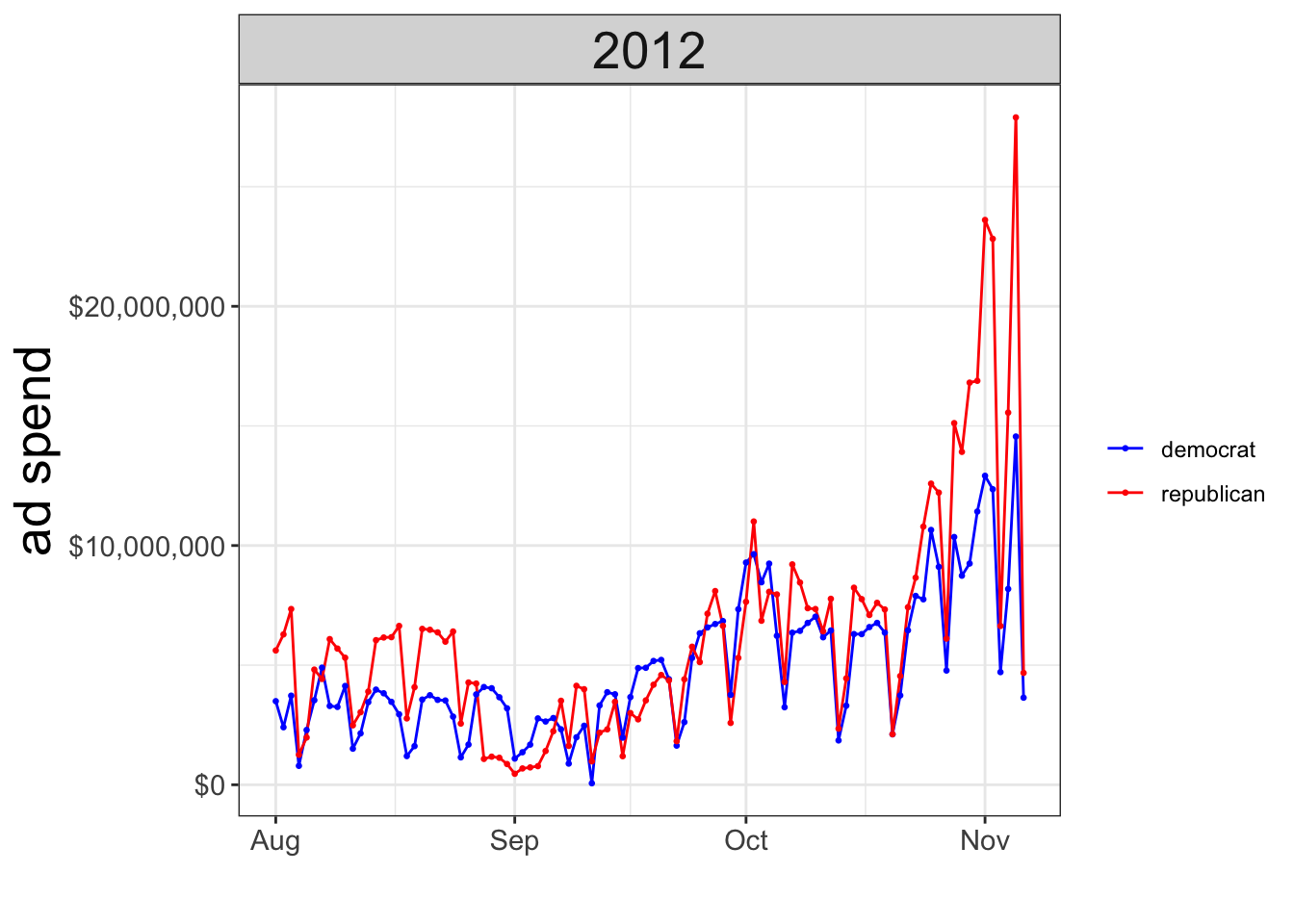
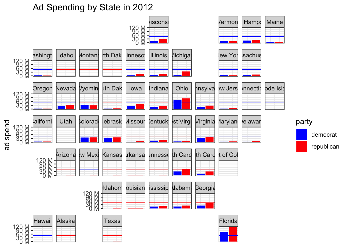
From these two graphs, we can observe that campaigns spend immense amounts of money on advertising and that this expense only increases as the election date nears. As reported by Open Secrets, TV ads are the single-largest expense of presidential campaigns, and the cost of presidential elections has only ballooned in recent cycles. The cost of the 2020 presidential election was near $5.7 billion (Open Secrets). The bulk of this spending is also concentrated in more competitive swing states.
Given the sheer volume of money that is spent on presidential elections, I am interested in constructing a regression to measure if there is any statistically significant relationship between campaign spending and two-party vote share. I will focus on the Democratic aisle between 2008 and 2020 using campaign spending data from the FEC.
| Dependent variable: | |||
| D | |||
| (1) | (2) | (3) | |
| Log(Contribution Amount) | 4.659*** | 1.091 | 0.343 |
| (0.460) | (0.678) | (1.234) | |
| State Fixed Effects | No | Yes | Yes |
| Year Fixed Effects | No | No | Yes |
| Observations | 200 | 200 | 200 |
| R2 | 0.341 | 0.938 | 0.959 |
| Adjusted R2 | 0.338 | 0.918 | 0.944 |
| Note: | *p<0.1; **p<0.05; ***p<0.01 | ||
While this is admittedly a very rough regression table, it is still telling that, even before controlling for time and entity fixed effects, the effect of campaign spending on democratic vote share is exceptionally minimal. And, once we have considered these two fixed effects, the effect of campaign spending is no longer statistically significant. This isn’t to suggest that advertisement spending is not consequential — it more likely evidences how campaign spending is like an arms race where the spending of one party is negated by the spending of the other.
Improving My Electoral College Model
Last week, I constructed an elastic model of the 2024 election using both fundamental and polling data.
This week, I will modify this model by exploring a Bayesian linear model in addition to the frequentist elastic net model. My elastic net model, this week, will be slightly different too as I will only consider the polling data from the past 8 weeks and I will not simultaneously predict both Republican and Democratic vote share. I am only considering polling data from the past 8 weeks as I believe constructing an “average polling average” for weeks when Biden was the nominee or before Harris had been cemented as the nominee could introduce inaccuracies to the projection. The Bayesian linear regression model will assume that the two-party Democratic vote share is normally distributed around the mean as calculate by the linear combination of the same variables initially included in the elastic net, and, then, I will construct a posterior distribution using Markov Chain Monte Carlo before ultimately offering a final prediction.
As was the case last week, I will use state-level polling average data since 1980 from FiveThirtyEight and national economic data from the Federal Reserve Bank of St. Louis. I will construct an elastic net model that uses the following fundamental and polling features:
- Latest polling average for the Democratic candidate within a state
- Average polling average for the Democratic candidate within a state
- A lag of the previous election’s two-party vote share for the Democrats within a state
- A lag of the election previous to last election’s two-party vote share for the Democrats within a state
- Whether a candidate was incumbent
- GDP growth in the second quarter of the election year
There are only 19 states for which we have polling averages for 2024. These 19 states include our 7 most competitive battleground states, a few other more competitive states, and a handful of non-competitive states (California, Montana, New York, Maryland, Missouri, etc.)
We will train a model using all of the state-level polling data that we have access to since 1980, and then test this data on our 19 states on which we have 2024 polling data. We can then evaluate how sensible the predictions are given what we know about each state.
Here are the results from our elastic-net model:
| state | simp_pred_dem | winner |
|---|---|---|
| arizona | 49.66918 | Republican |
| california | 61.23450 | Democrat |
| florida | 47.61852 | Republican |
| georgia | 50.22281 | Democrat |
| maryland | 64.67678 | Democrat |
| michigan | 50.74988 | Democrat |
| minnesota | 52.99454 | Democrat |
| missouri | 44.08608 | Republican |
| montana | 42.47695 | Republican |
| nevada | 50.09261 | Democrat |
| new hampshire | 53.89531 | Democrat |
| new mexico | 53.06882 | Democrat |
| new york | 56.44713 | Democrat |
| north carolina | 49.56832 | Republican |
| ohio | 45.53835 | Republican |
| pennsylvania | 50.31533 | Democrat |
| texas | 47.22080 | Republican |
| virginia | 53.50393 | Democrat |
| wisconsin | 50.43930 | Democrat |
And here are the predictions from our Bayesian linear regression model:
| state | bayes_pred_dem | bayes_winner |
|---|---|---|
| arizona | 49.54917 | Republican |
| california | 61.08212 | Democrat |
| florida | 47.46509 | Republican |
| georgia | 50.12053 | Democrat |
| maryland | 64.59000 | Democrat |
| michigan | 50.62747 | Democrat |
| minnesota | 52.89556 | Democrat |
| missouri | 43.97149 | Republican |
| montana | 42.36632 | Republican |
| nevada | 49.95889 | Republican |
| new hampshire | 53.80484 | Democrat |
| new mexico | 52.93385 | Democrat |
| new york | 56.27412 | Democrat |
| north carolina | 49.44359 | Republican |
| ohio | 45.39828 | Republican |
| pennsylvania | 50.19036 | Democrat |
| texas | 47.09954 | Republican |
| virginia | 53.40320 | Democrat |
| wisconsin | 50.30651 | Democrat |
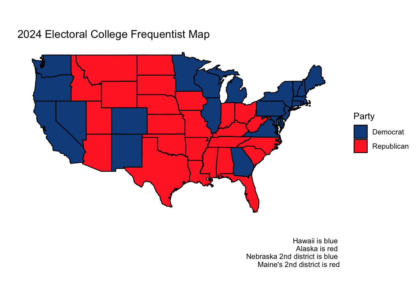
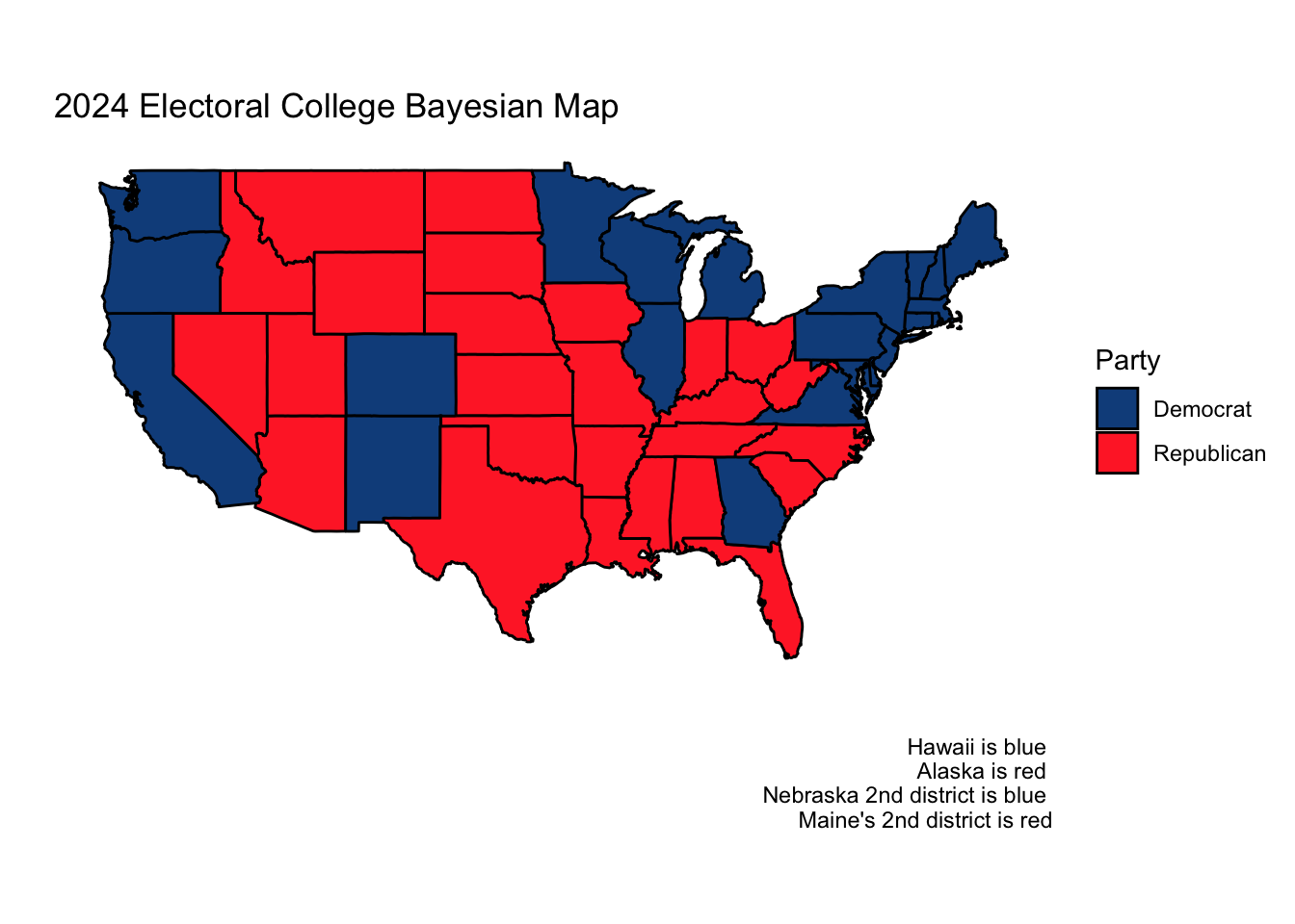
Apart from slightly different polling predictions, the only significant departure in this Bayesian prediction from the frequentist prediction is the winner of Nevada, which, per the Bayesian model, is Trump.
These electoral maps are visible below.
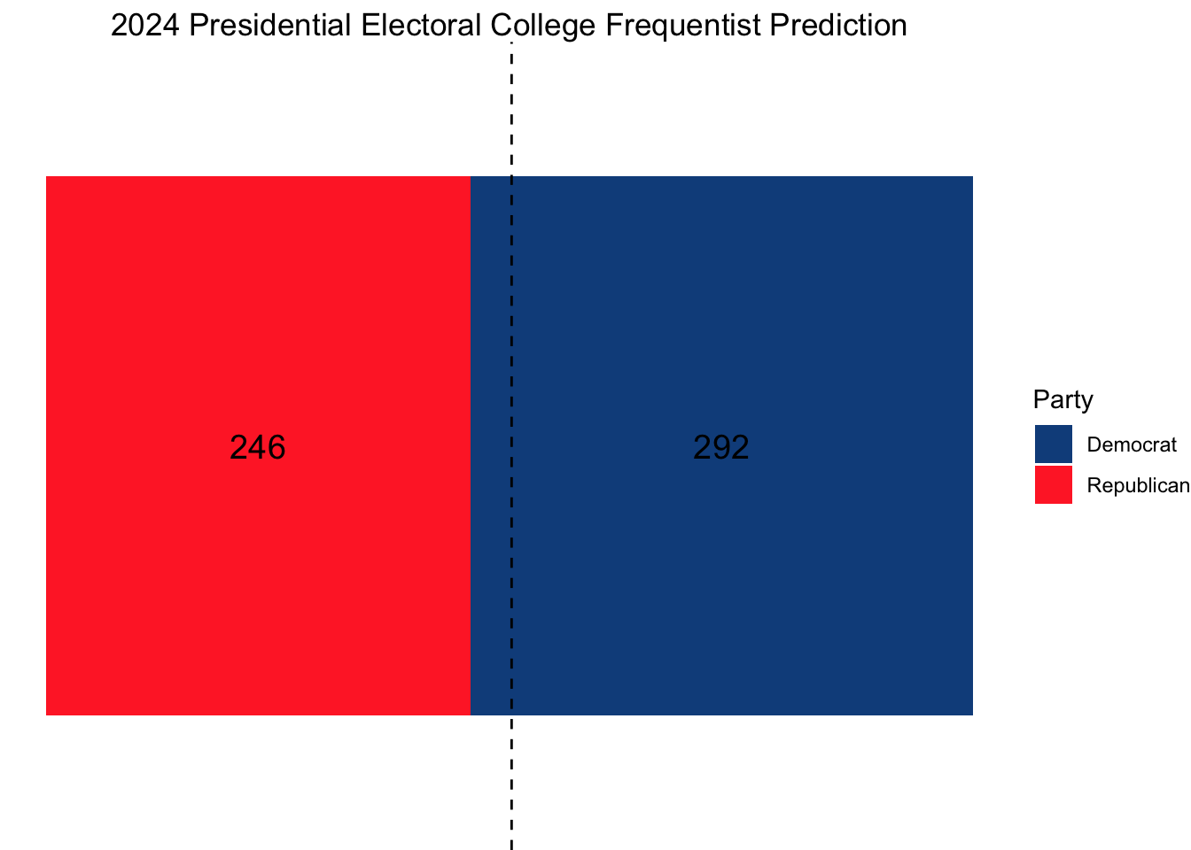
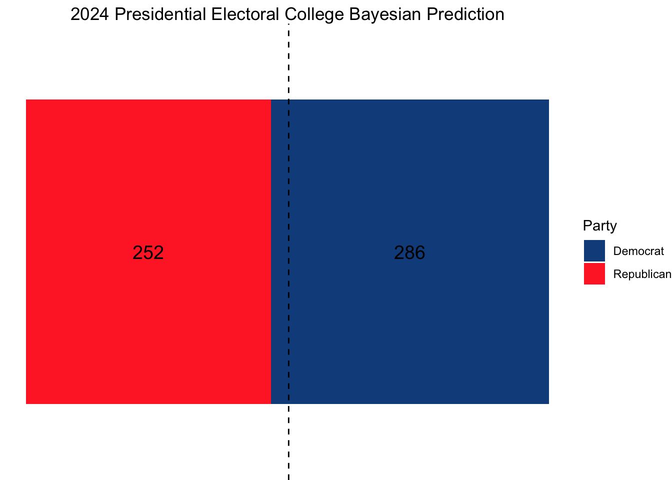
If we also wanted to model the national popular vote, we could use what we did in Week 3, using an elastic net on both fundamental and polling data, weighting such that the polls closer to November matter more. This was Nate Silver’s approach. Again, I will only be considering polls within 8 weeks of the election.
Doing so, we find that the Democrats are projected to have a narrow lead in the two-party popular vote nationally (after scaling so that the estimates sum to 100%).
## Democrat two-party vote share: 50.93 %
## Republican two-party vote share: 49.07 %
Citations:
Cavazos, Nidia, et al. “Kamala Harris Campaign Surpasses $1 Billion in Fundraising, Source Says.” CBS News, CBS Interactive, 10 Oct. 2024, www.cbsnews.com/news/kamala-harris-campaign-fundraising-1-billion/.
Evers-Hillstrom, Karl. “Most Expensive Ever: 2020 Election Cost $14.4 Billion.” OpenSecrets News, 11 Feb. 2021, www.opensecrets.org/news/2021/02/2020-cycle-cost-14p4-billion-doubling-16/.
Kamarck, Elaine, et al. “Why Hillary Clinton Lost.” Brookings, 20 Sept. 2017, www.brookings.edu/articles/why-hillary-clinton-lost/.
Data Sources:
Data are from the US presidential election popular vote results from 1948-2020, polling data from fivethirtyeight, economic data from the St. Louis Fed, campaign spending data from the FEC between 2008 and 2024, and campaign advertisement data from the Wesleyan Media Project.