Introduction
In this seventh blog post, I am going to explore the use of logistic regression as opposed to linear regression while creating my models and simulations and evaluate how my electoral college projections change.
My projections from last week (which used elastic net linear regression) are available here.
The code used to produce these visualizations is publicly available in my github repository and draws heavily from the section notes and sample code provided by the Gov 1347 Head Teaching Fellow, Matthew Dardet.
Analysis
Though linear regression is an accessible, easy-to-use modelling tool with interpretable coefficients, there exist reasons to believe that it might be a less suitable regression model compared to logistic regression when it comes to polling. Here are a couple.
Issues with Extrapolation:
In linear regression, there is no guarantee that a predicted vote share will fall between 0 and 100. OLS regression is simply minimizing the residual sum of squares, meaning that, if new data falls outside of what has historically been observed, we run the risk of extrapolating the outcome of that new observation to a value that is nonsensical. Logistic regression, on the other hand, bounds all predictions within a range. In our case, where we are predicting a given party’s two-party vote share given its polling average, this prediction would be between 0 and 100.
Probability-based Framework
In many ways, using logistic regression makes intuitively more sense in the context of an election. In the case of two-party vote share, each person’s vote is necessarily binary: they either vote Republican or Democrat. The total number of trials is also fixed in a given year, this value being equivalent to the fraction of the voting-aged population that turns out. Given that logistic regression models the probability of a “success” in any trial, logistic regression is arguably better suited to be applied to the data.
Visualizations
Provided these reservations, I am motivated to explore logistic regression.
Below, we have two graphs: A map of the United States made with linear regression models, and a side-by-side comparison of the linear regression models in California and Florida.
These linear models have, on the x-axis, the hypothetical poll support for the Republican and Democratic party (depending on which line, red or blue you are looking at), and, on the y-axis, the predicted two-party vote share for each party. These linear regressions were created by analyzing the polling averages and two-party vote share outcomes for every state’s presidential election since 1980. We will be looking at the polling average in each state up to 8 weeks before the presidential election.
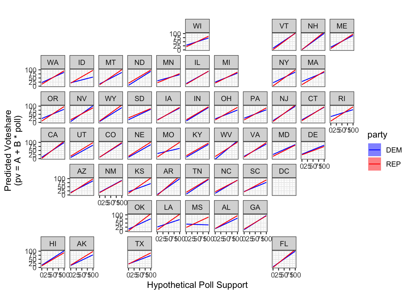
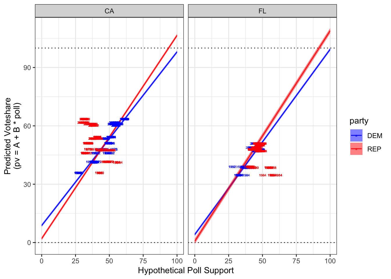
As we can see in the graphs, the lines constructed through linear regression are not bounded by 0% and 100%. If, for example, a Republican were to be running in California with a 90+% polling average, we would project that he/she would garner over 100% of the vote, which is not possible. Similarly, there exists a negative sloping line for Democrats in Mississippi, which is the opposite of what we would logically expect.
Now, let’s see if we can correct this by using logistic regressions instead.
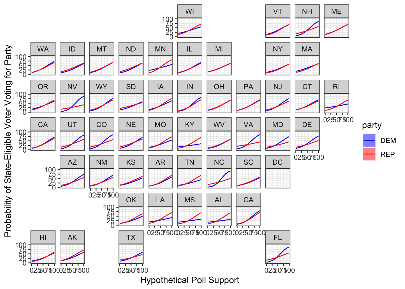
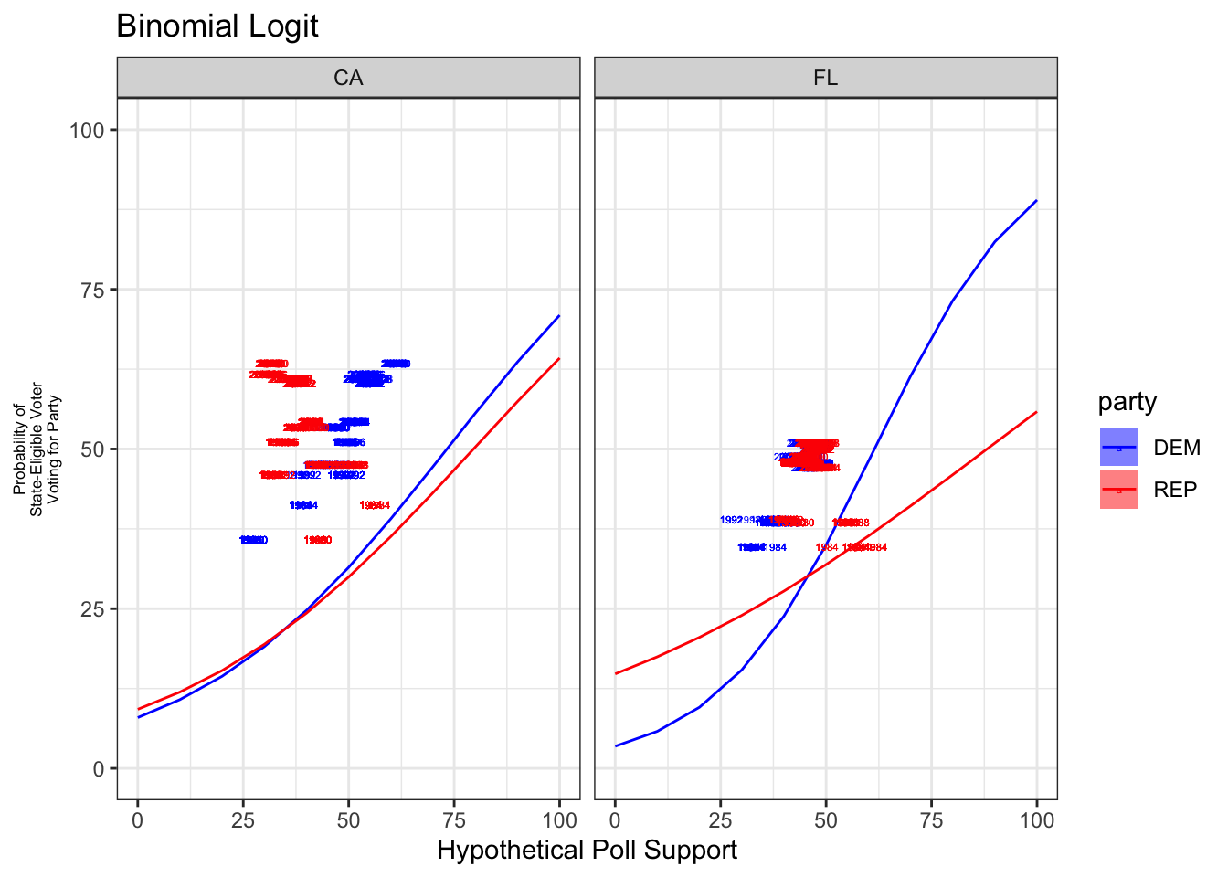
This time, using logistic regression instead of linear regression, we get the following graphs that do not exhibit the same extrapolation issues. Here, we should be careful to note that our logistic regression is modeling the probability of a state-eligible voter voting for each party. Since this is a probability between 0 and 100% and not a measure of two-party vote share, we should not be concerned that the points do not line up with the graphs.
Simulations
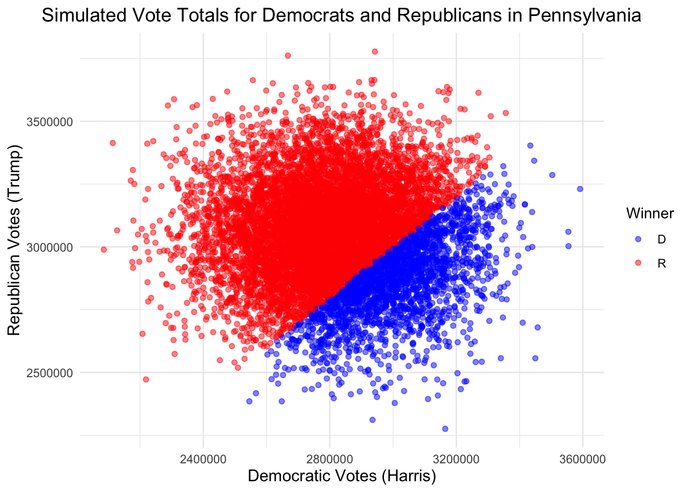
Now that we have a measure of the probability of a state-eligible voter voting for each party, we can run simulations to produce a distribution of the number of votes cast for each candidate. Let’s do this first with Pennsylvania, for example.
First, let’s plot the historical voting-eligible population in Pennsylvania using historical voter turnout data.
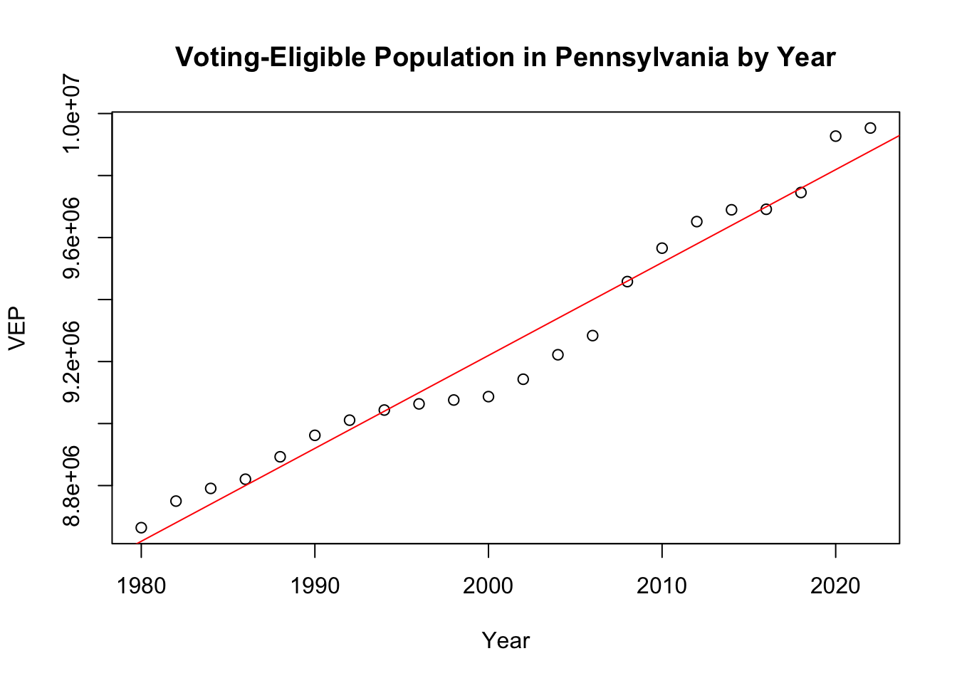
Rather than apply a linear model to something that appears visibly non-linear, let’s use a general additive model that employs splines to fit the data.
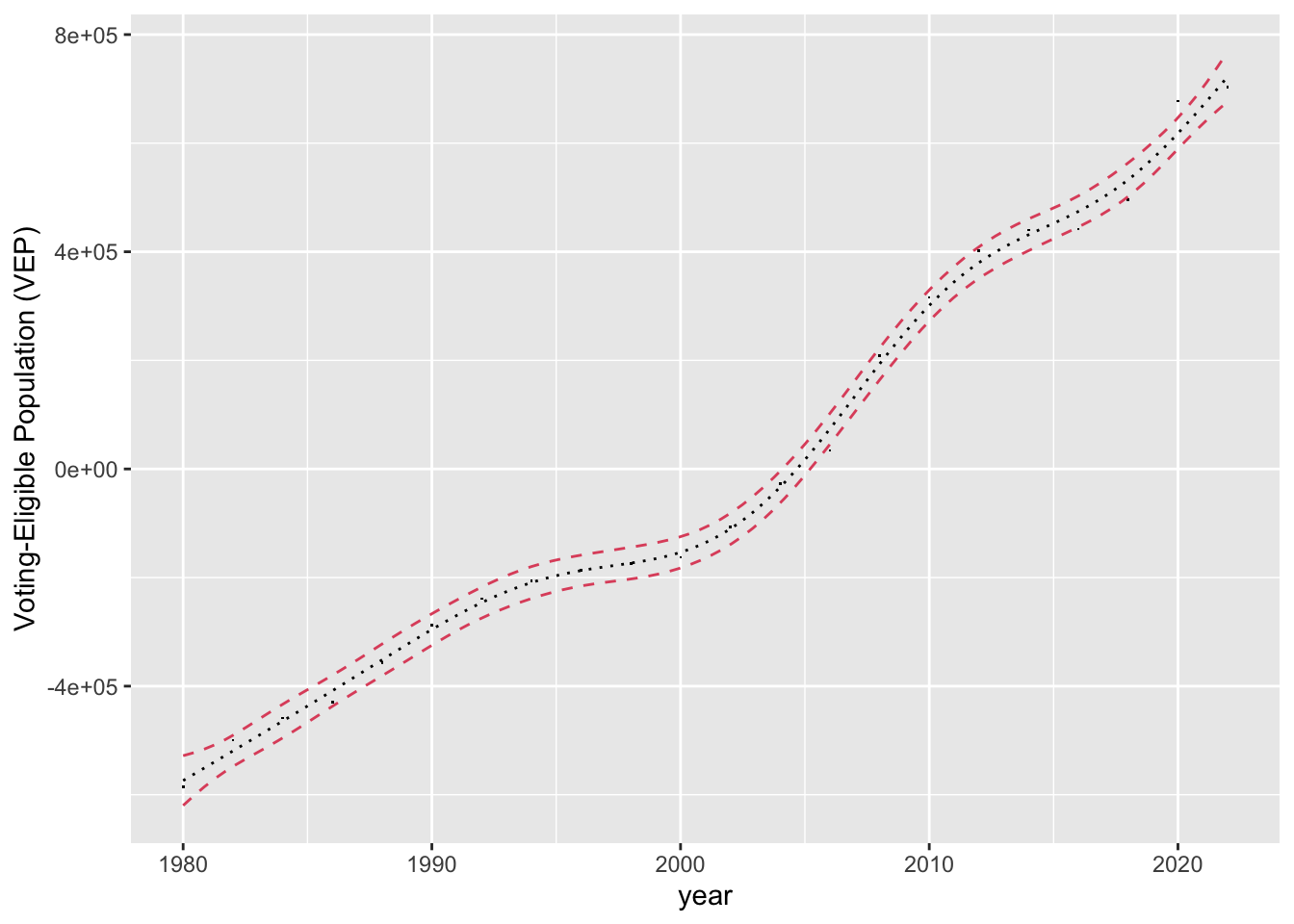
We take a weighted 75:25 weighted average of the GAM model and OLS model to get a predicted VEP population for 2024. With this VEP population, we can fit two logistic models, one for Republicans and another Democrats, to estimate the probability of a stte-eligible voter voting for each party’s candidate based on that candidate’s average polling support over the last 60 days.
After running our code, we find that, given our current polling average of 47.9% for Democrats and 47.05% for Republicans, given the historical data and the logistic model, we can expect a state-eligible voter to vote for a Democrat 27.9% of the time and a Republican 29.9% of the time. This would align with the narrative that Democrats tend to underperform relative to the polls in Pennsylvania.
We can then run a simulation to estimate the number of votes that each candidate will receive given the calculated predicted probabilities and a 2 percentage-point standard deviation.
| Candidate | Simulations Won |
|---|---|
| D | 2198 |
| R | 7802 |
We observe that, according to this model, Harris would lose Pennsylvania in the majority of our simulations.
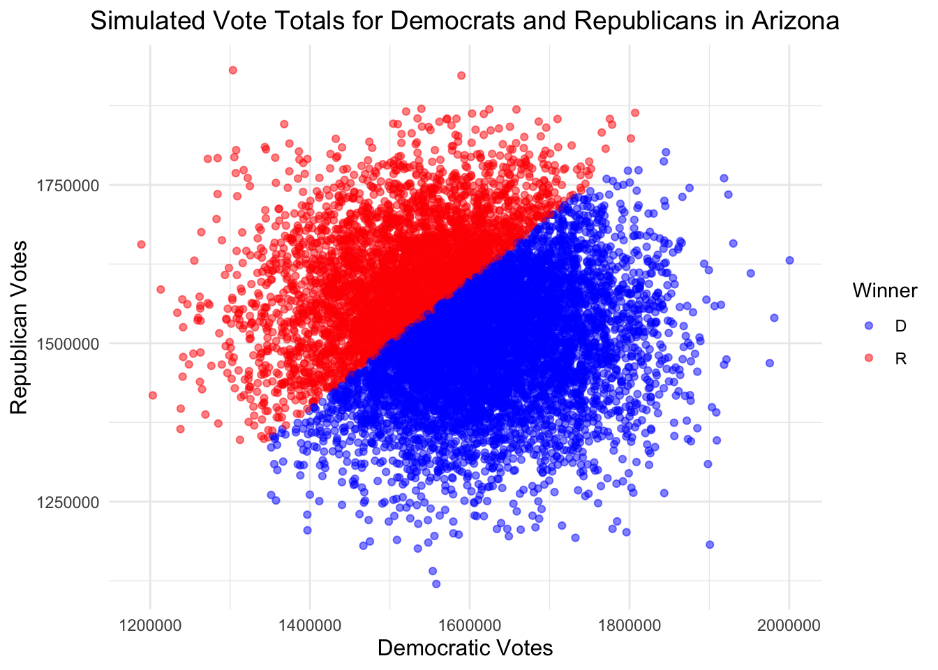
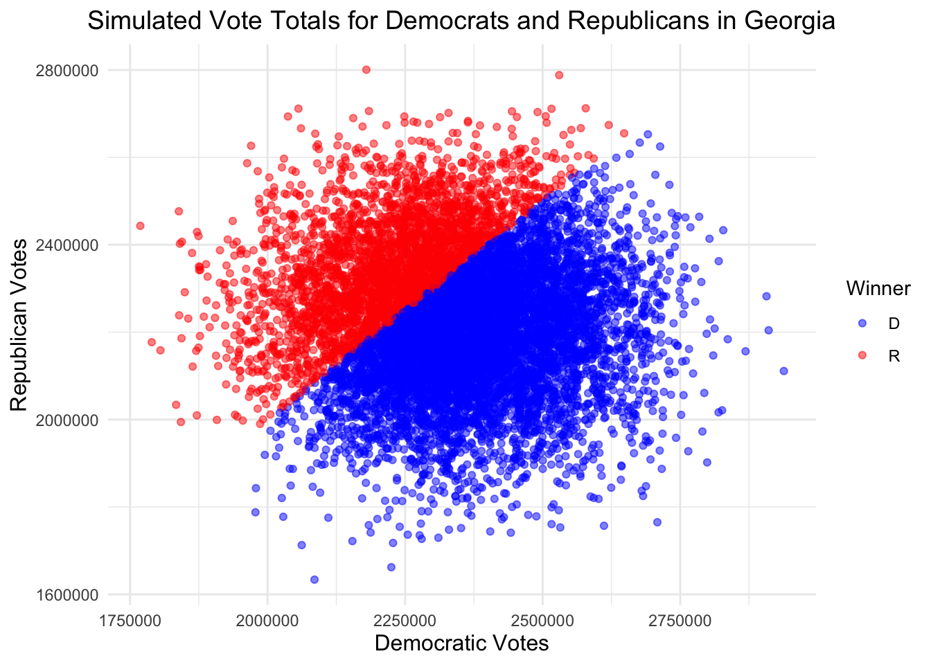
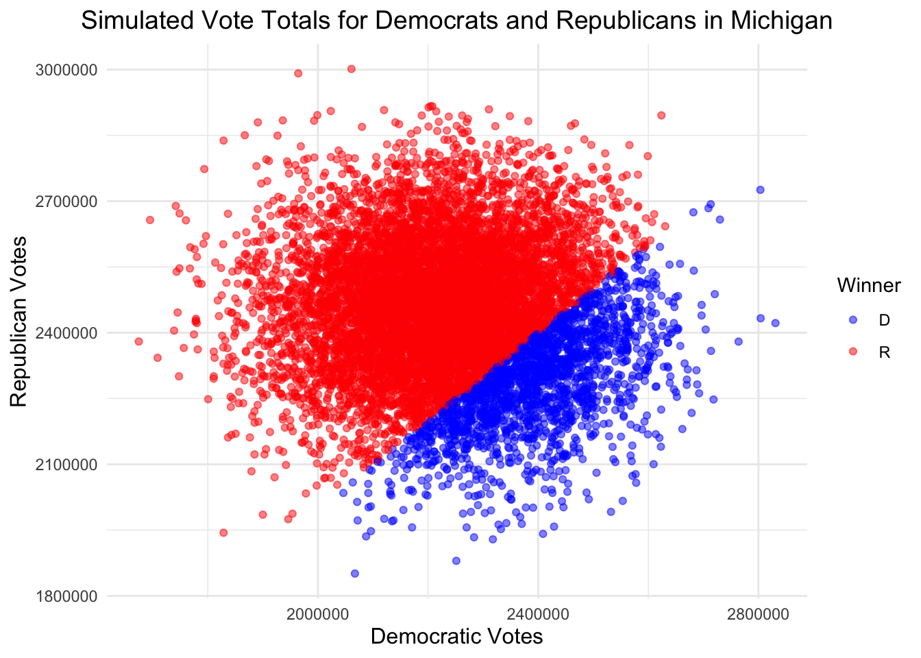
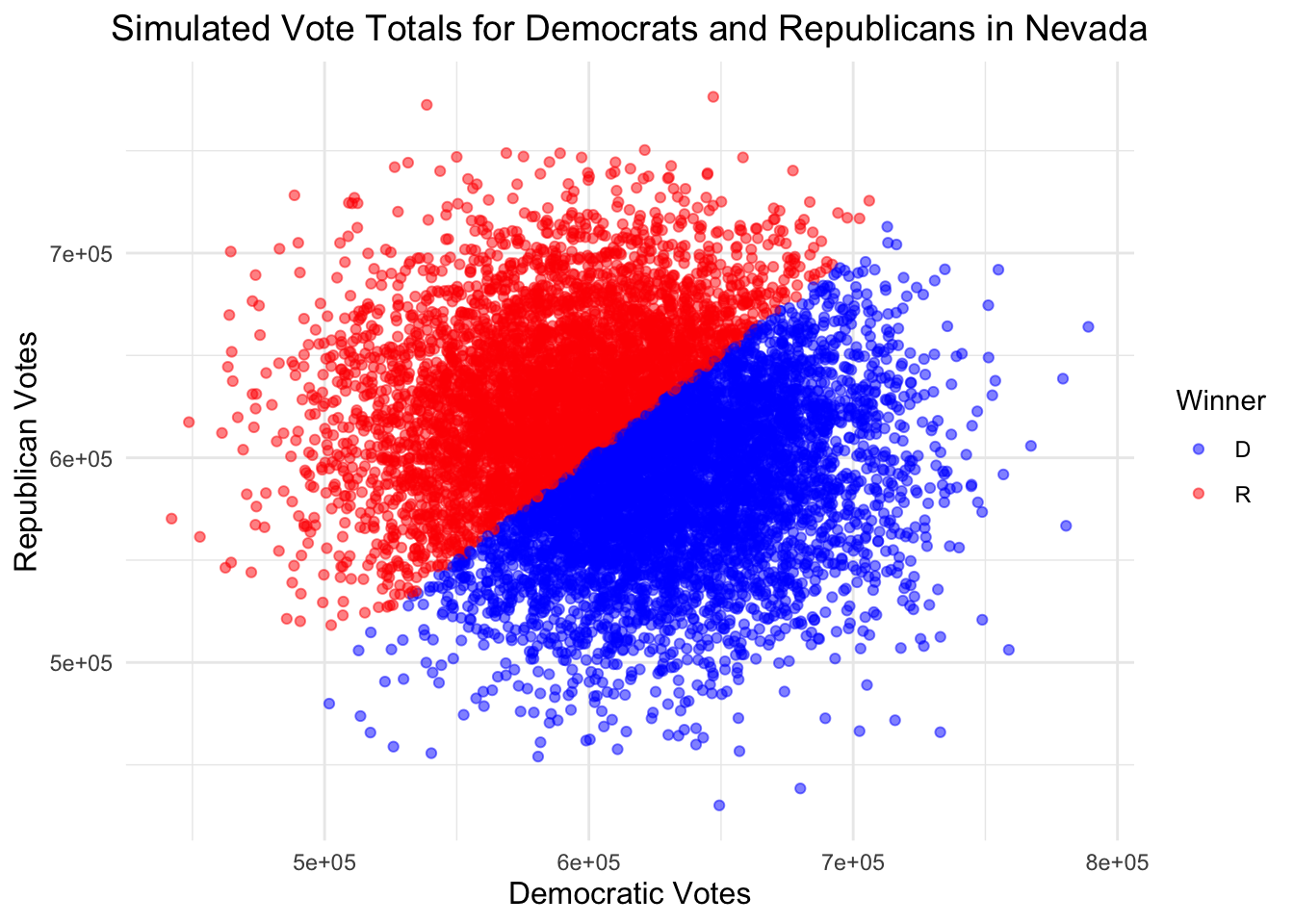
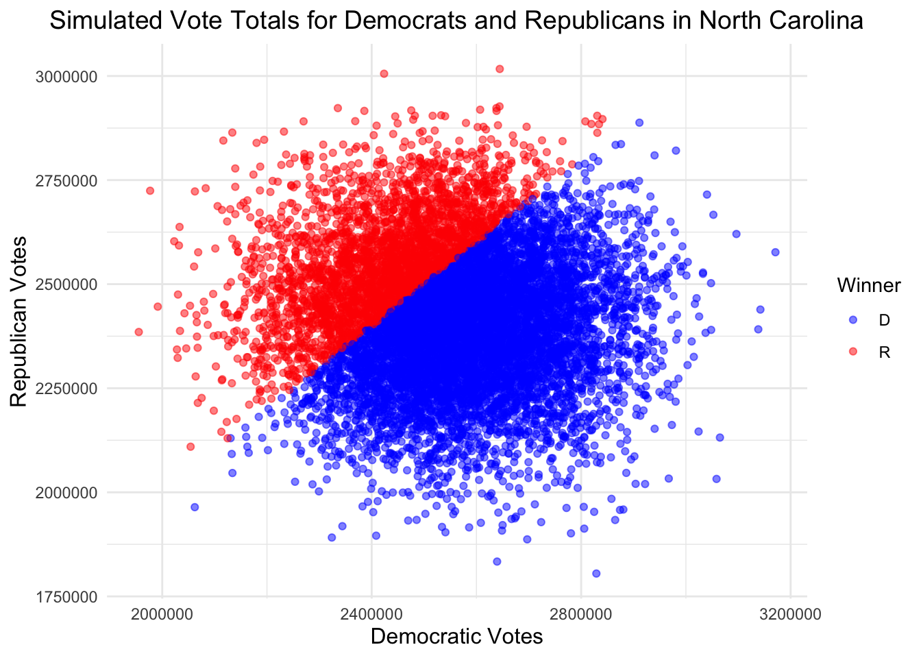
If we do this same thing for our other six swing states (Arizona, Georgia, Michigan, Nevada, North Carolina, and Wisconsin), we get the following graphs.
| Candidate | Simulations Won |
|---|---|
| D | 6250 |
| R | 3750 |
| Candidate | Simulations Won |
|---|---|
| D | 6929 |
| R | 3071 |
| Candidate | Simulations Won |
|---|---|
| D | 1851 |
| R | 8149 |
| Candidate | Simulations Won |
|---|---|
| D | 5302 |
| R | 4698 |
| Candidate | Simulations Won |
|---|---|
| D | 7070 |
| R | 2930 |
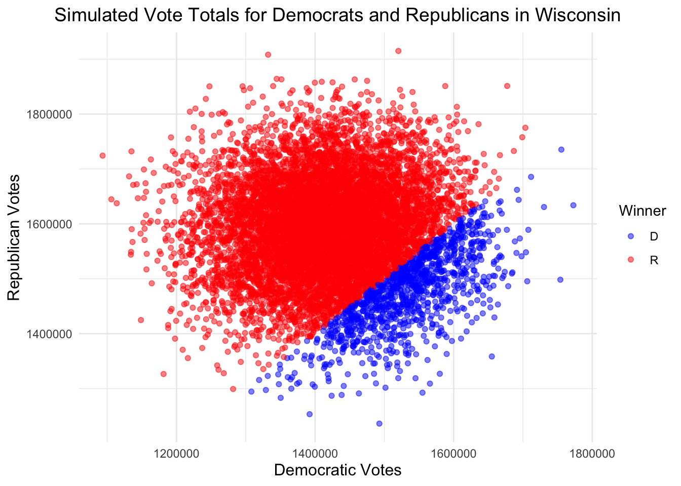
| Candidate | Simulations Won |
|---|---|
| D | 1167 |
| R | 8833 |
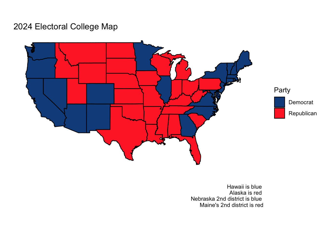
These simulations indicate Harris victories in Arizona, North Carolina, Georgia, and Nevada, and Trump victories elsewhere.
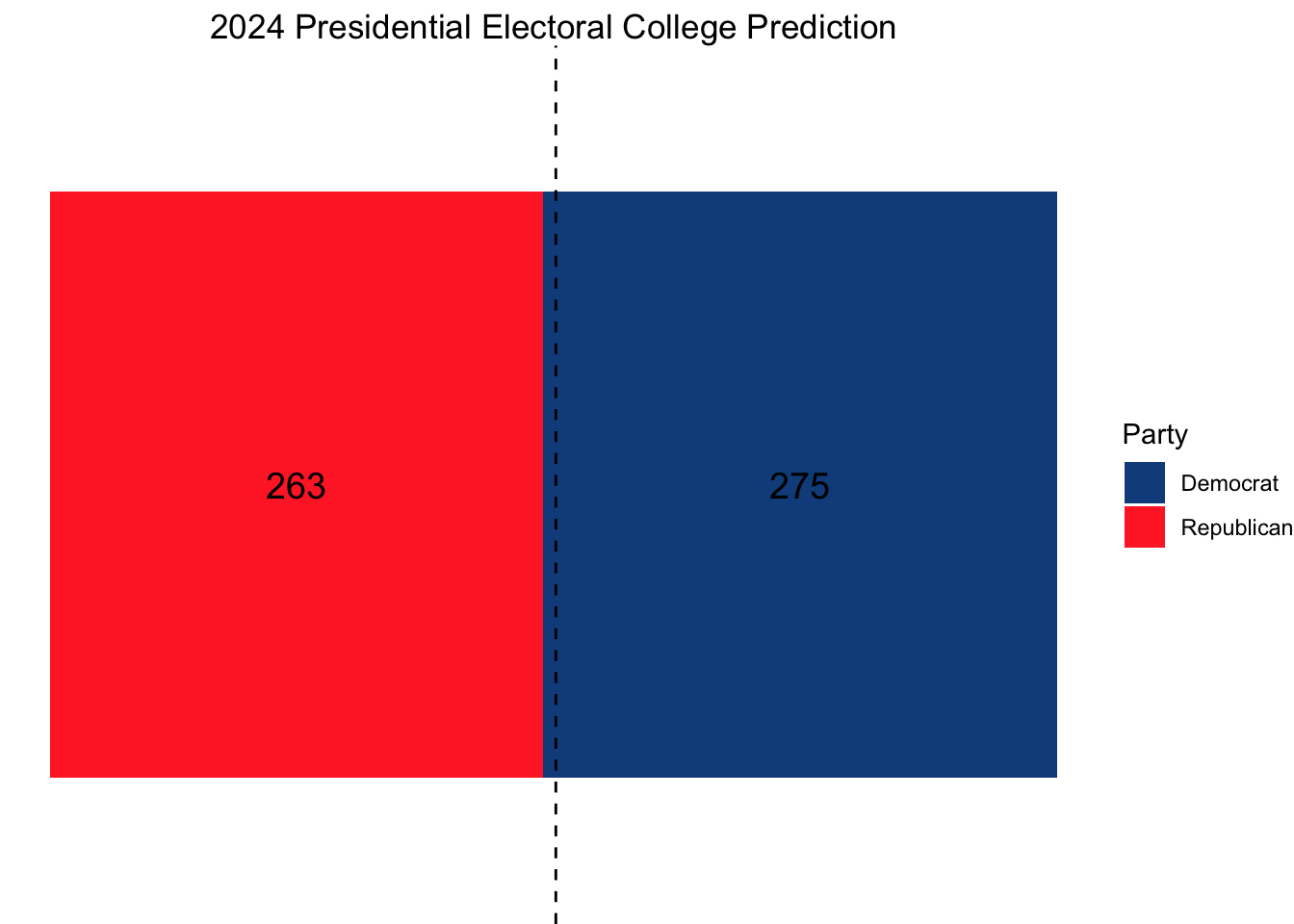
Ultimately this would result in the following electoral college map in Harris’s favor.
Citations:
Kanade, Vijay. “Linear vs. Logistic Regression.” Spiceworks Inc, 10 June 2022, www.spiceworks.com/tech/artificial-intelligence/articles/linear-regression-vs-logistic-regression/.
Data Sources:
Data are from the US presidential election popular vote results from 1948-2020, polling data from fivethirtyeight and voter turnout (VEP) data from the University of Florida’s Election Lab.