Introduction
In this post-election blog post, I am going to do the following:
Provide a recap of my model and the predictions it generated
Assess the accuracy of my model and look for patterns in the accuracy
Hypothesize why the model diverged from the actual results
Propose some quantitative tests that could assess my hypotheses.
Offer a description of how I would approach the model differently now if I were to do it again.
The code used to produce these visualizations is publicly available in my github repository and draws heavily from the section notes and sample code provided by the Gov 1347 Head Teaching Fellow, Matthew Dardet.
Model Recap
First, I will summarize my model:
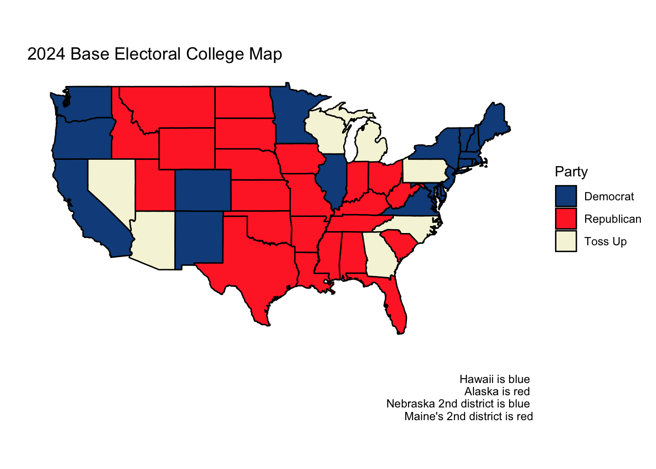
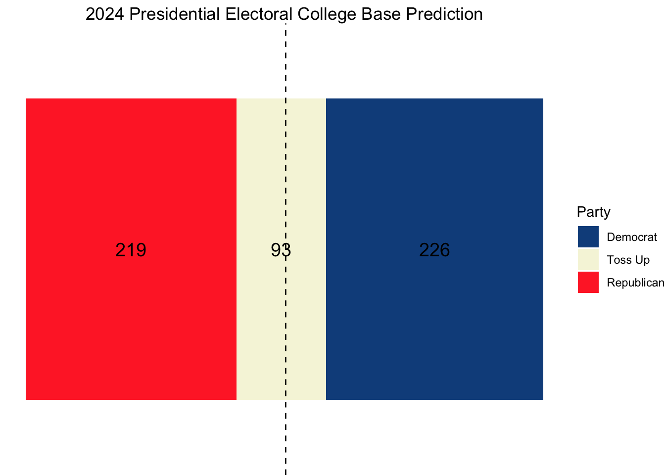
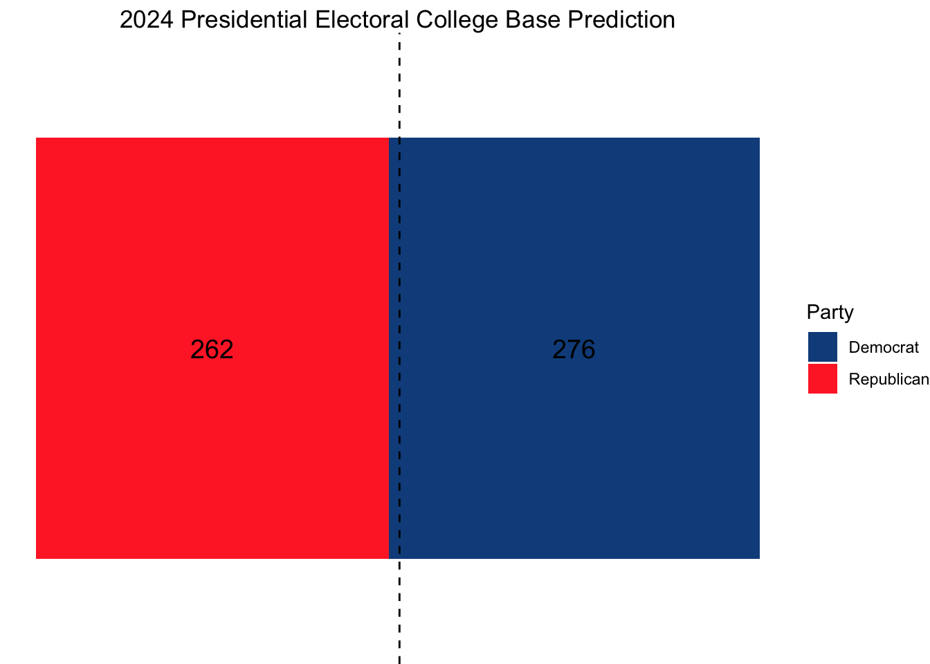
Based on assessments from Sabato’s Crystal Ball of the Center for Politics and the Cook Political Report, I conjectured that the seven states of Arizona, Georgia, Michigan, Nevada, North Carolina, Pennsylvania, and Wisconsin would be the most competitive and elected to focus my model on them while assuming that the other states (and districts) would vote as they did in 2020.
This gave us the following initial electoral college map:
From here, I used national-level polling average data since 1968 from FiveThirtyEight to predict the national two-party vote share. Specifically, I took the national polling averages for the Republican and Democratic candidates in each of the ten weeks preceding the election and then rescaled the Democratic average to be a two-party vote share. After doing this, I used leave-one-out cross validation across the elections from 1972 to 2020 to find the optimal decay factor to weight each of the national polling averages in the 10 weeks leading up to election day. For example, a decay factor of 0.9 would mean that the polling average immediately before the election would have a weight of 0.9^(1-1) = 1, the polling average two weeks before the election would have a weight of 0.9^(2-1) = 0.9, the polling average three weeks before the election would have a weight of 0.9^(3-1) = 0.81, etc. After performing cross-validation to uncover the optimal decay value of 0.78, I used this decay factor to find the weighted average of the 2024 national- and swing state-level polls in the 10 weeks leading up to the election.
This produced the following national and state-level predictions:
National Popular Vote Prediction
| Year | Predicted Democratic Two-Party Vote Share | Predicted Republican Two-Party Vote Share |
|---|---|---|
| 2024 | 51.15365 | 48.84635 |
State-level Predictions
| State | Predicted Democratic Two-Party Vote Share |
|---|---|
| Arizona | 49.24514 |
| Georgia | 49.36078 |
| Michigan | 50.57455 |
| Nevada | 50.19946 |
| North Carolina | 49.56858 |
| Pennsylvania | 50.18314 |
| Wisconsin | 50.53039 |
To get a sense of the certainty we had in our weighted polling average predictions, I produced a simulation that sampled new state-level polling measurements for each of our 7 states 10,000 times, assuming a normal distribution around the weighted polling average with a standard deviation determined by the stein-adjusted average distance of each state’s poll away from the actual outcome in the 2016 and 2020 elections.
| State | Average Error | Stein Adjusted Error |
|---|---|---|
| Arizona | 1.5458014 | 1.7387023 |
| Georgia | 0.4857592 | 0.9464523 |
| Michigan | 3.5667802 | 3.2491329 |
| Nevada | 1.1831851 | 1.4676916 |
| North Carolina | 2.3973182 | 2.3751053 |
| Pennsylvania | 3.1957976 | 2.9718696 |
| Wisconsin | 3.7910859 | 3.4167736 |
This produced the following distribution of simulations:
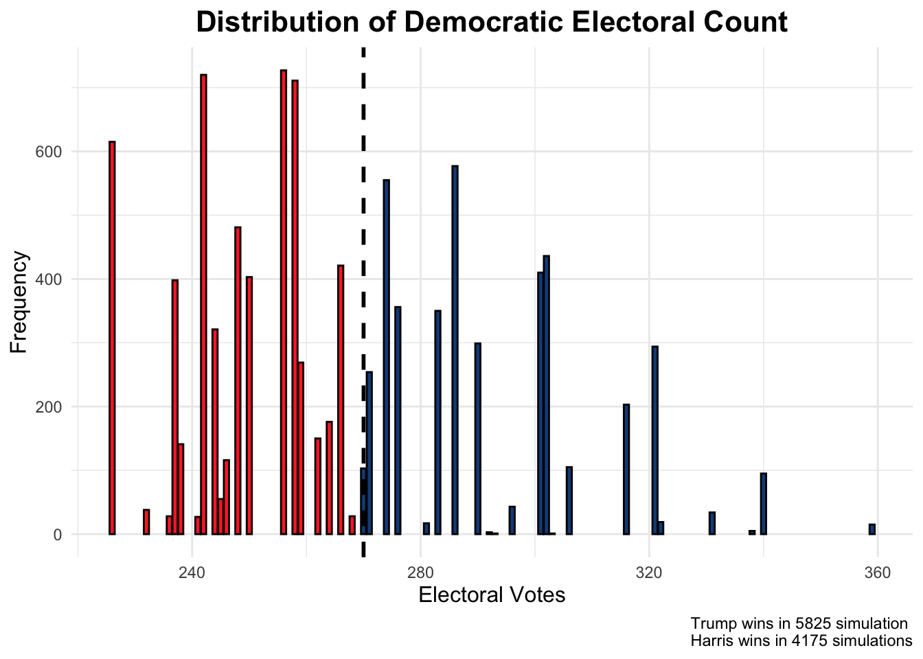
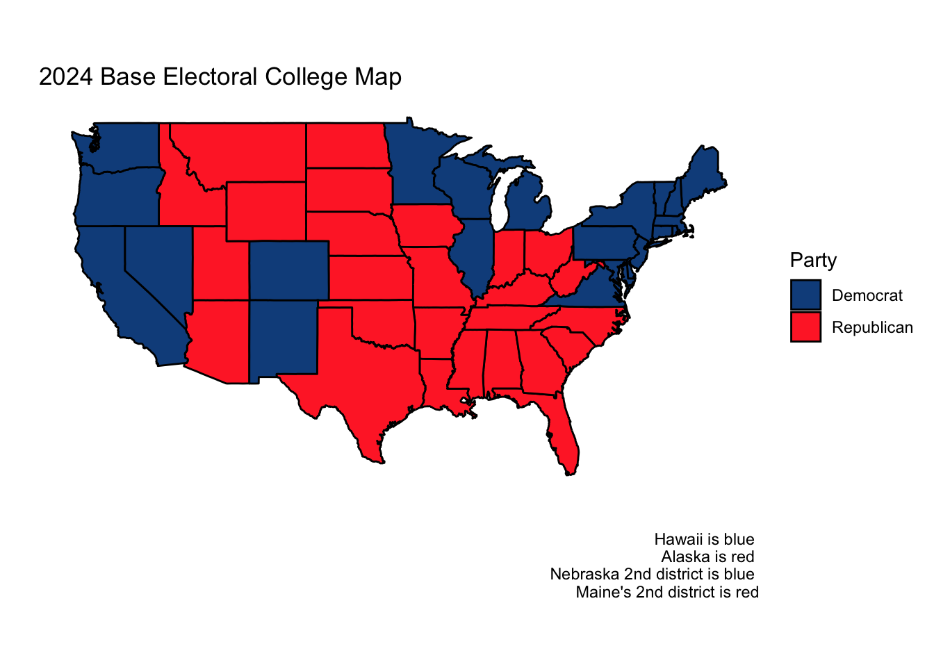
While the overall prediction was a Trump win in 58% of the simulations, predicting each state separately resulted in a narrow win projection for Harris.
Model Assessment
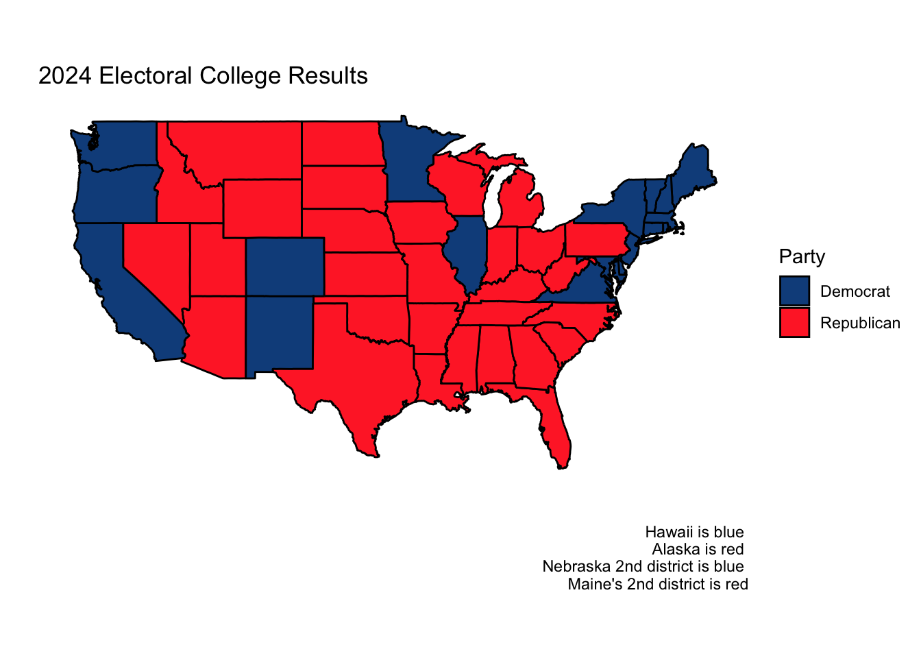
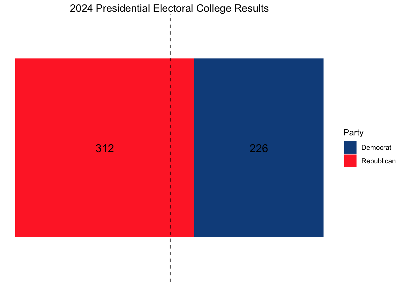
For anyone familiar with the results of the 2024 election, it is obvious that my model was inaccurate in many ways. Below are the actual electoral college and two-party popular vote results (national and state).
| State | Actual Dem Two-Party Vote Share | Predicted Dem Two-Party Vote Share | Error |
|---|---|---|---|
| Arizona | 47.15253 | 49.24514 | 2.0926146 |
| Georgia | 48.87845 | 49.36078 | 0.4823282 |
| Michigan | 49.30156 | 50.57455 | 1.2729947 |
| Nevada | 48.37829 | 50.19946 | 1.8211677 |
| North Carolina | 48.29889 | 49.56858 | 1.2696834 |
| Pennsylvania | 48.98235 | 50.18314 | 1.2007949 |
| Wisconsin | 49.53156 | 50.53039 | 0.9988300 |
| National | 48.88896 | 51.15365 | 2.2646945 |
While my prediction that no state or electoral district outside of the 7 swing states would flip from how it voted in 2020 turned out to be true, I inaccurately predicted four of the seven swing states, a majority. Likewise, my 2024 state predictions had an RMSE of 1.39. While this is not a very high RMSE, upon reflection, I can think of many ways I could have reduced it.
Interestingly, we see that our predicted two-party Democratic vote share was consistently greater than the actual two-party Democratic vote share in each of our states. In other words, in every one of our predictions, we overestimated the two-party Democratic vote share. I knew that the polls overestimated Democratic support in both 2016 and 2020 in every one of our seven swing states (except in Nevada in 2016), but I was hesitant to assume that the polls in 2024 were overestimating Democratic support again. I didn’t want to make too many assumptions off of a sample size of two. Looking at these results, however, I wish I had assumed the 2024 polls were overestimating Democratic support similarly to how they had in 2016 and 2020 in those same states. Had I done so, I would have predicted every state correctly. Instead, I assumed the distribution of the 2024 polling errors would be independent across states, symmetric about 0, and have a standard deviation of the stein-adjusted average of the absolute value of the 2016 and 2020 polling errors based on my model.
I want to visualize the 2016, 2020, and 2024 errors. This error will be calculated as the difference between what my model predicted for each year (the weighted two party vote share average) and the actual Democratic two-party vote share. I will also include the stein-adjusted error that I prepared in my election model (for the national model, the stein-adjusted error is just the average error between 2016 and 2020).
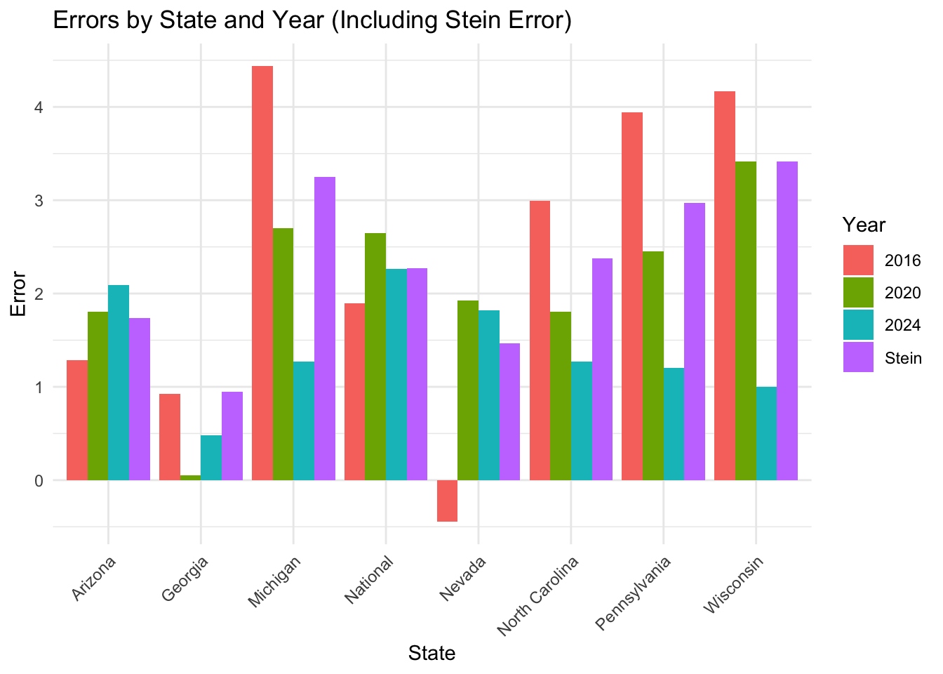
Looking at the 2024 errors, a few patterns emerge. Most states saw either year-to-year increases or decreases in polling error, the exceptions being Georgia, Nevada, and the nation as a whole. This suggests to me that we could have used a stein-adjusted linear regression to have predicted the 2024 polling error using the polling errors in 2016 and 2020. Moreover, our stein-adjusted polling error estimator had an RMSE of 2.472053, which was slightly larger than the actual RMSE. Had I used the stein-adjusted polling error to shift my predicted two-party vote share down instead of using it solely to estimate standard deviations, I would have correctly predicted the outcome of each state and nearly PERFECTLY estimated the national two-party vote share.
I have some hypotheses for why my model diverged from the actual results.
Firstly, I think there was an element of partisanship affecting the modelling. In my own case, in earlier weeks, I had used elastic net models to perform feature selection and weighting on a variety of polling, economic, and fundamental variables. While I observed that the RMSE was minimized when RDPI (real disposable income) was included, the accompanying prediction that all swing states would shift red did not match my prior on how I thought (and hoped) the election would turn out. In other words, my own hopes that Harris would win may have subconsciously affected my willingness to entertain models that showed Trump winning commandingly. One way that I could test this hypothesis is by looking at the relationship between other students’ predictions and partisan affiliations. This might entail preparing a logistic regression that models the projected winner of the 2024 election with a sliding scale for political ideology and then evaluating whether the coefficient on the sliding scale variable is statistically significant. While I do not have data on my peers’ political affiliations, the fact that over 75% of my classmates predicted a Harris win when pollsters were generally predicting a toss-up election suggests to me that there is strong evidence of bias among my classmates (since it is well-known that most students at Harvard are left-leaning). I think my own prior that the election would be close also prevented me from assuming the polling errors would swing toward Trump just as they did in 2016 and 2020, another liability in my model in addition to the exclusion of fundamental/economic variables.
In terms of why the polling averages weren’t sufficiently accurate, or why the polling error in Republicans’ favor existed, I am curious if there was greater excitement among Republicans than Democrats. This excitement could manifest itself in turnout data, so I could prepare a logistic regression to evaluate if registered Republicans were more likely to vote than registered Democrats, even after controlling for various demographic variables.
Lastly, I am curious if polling methodology systematically undercounts Trump supporters. One way to explore this conjecture would be to collect metadata on how all the various 2024 surveys were conducted and then use machine-learning methods like PCA decomposition to match similar methodologies together. I am curious if there are certain methods like in-person polling that are more likely to collect the responses of working-class voters who might not answer the phone and systematically vote for Trump in greater numbers. I could test this by evaluating whether there are statistically significant differences in polling averages among decomposition groups, perhaps using an ANOVA test.
If I were to model the election again, I would do several things
- Not assume that the weighted polling average was unbiased. I would use data from the Trump era (2016 and 2020) to estimate how far off the 2024 prediction would be in each state. This could take the form of a stein-adjusted linear regression.
- I would have prepared an elastic net model that used polling averages, economic variables, and fundamentals, and let the computer perform feature selection for me as it calculated which model produced the smallest RMSE. I also would have weighted the models’ performance in 2016 and 2020 higher.
- I would have adjusted my simulation to allow for correlation between states.
Citations:
Teichholtz, Leah J., and Meimei Xu. “National Politics.” The Harvard Crimson’s 2024 Senior Survey, The Harvard Crimson, 2024, https://features.thecrimson.com/2024/senior-survey/national-politics/. Accessed 17 Nov. 2024.
Data Sources:
Data are from the US presidential election popular vote results from 1948-2024 and state-level polling data for 1968 onwards.